4. Motion and alignment plans

4.1. Generic motor scans

The alignment chores discussed below are implemented as specialized applications of a generic linescan. A linescan is when you move a motor and plot the signal on a detector.

At BMM, you can make a linescan using almost any motor on the beamline, including coordinated virtual axes such as slits.hcenter (see Section 2.2) or table.vertical (see Section 2.4). Any detector discussed in Section 3 can be plotted during the linescan.

The syntax of a linescan is

RE(linescan(motor, detector, start, stop, nsteps))

where

motor:

The name of the motor, any name given in Section 2, Motors and Coordinated Motions

detector:

A string indicating the signal from a scalar or a detector ROI, as discussed in Section 3, Detectors

start:

The starting point of the scan, in relative units from the current position of the motor (an integer or float)

start:

The stopping point of the scan, in relative units from the current position of the motor (an integer or float)

nsteps:

The number of steps in the scan (an integer)

After a scan is finished, the user is prompted to “pluck” a point from the plot. If you respond y or simply hit Enter, you have 20 seconds to click on a spot on the plot. A second prompts then verifies that you clicked correctly before moving the motor from the linescan to the selected point.

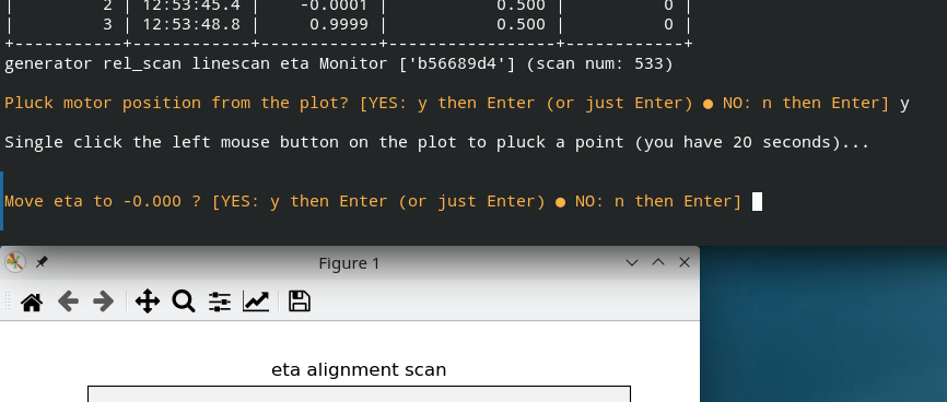
Fig. 4.1 The on-screen prompt to pluck a position from the linescan that just finished.

You can redo this point selection followed by motor motion with any plot still on screen. Simply do

RE(pluck())

then follow the prompts.

4.2. Direct beam camera

Attach the mounting bracker for the direct beam camera to its mount point on the floor, as shown in Figure 4.2. When securing the mounting bracket to the floor, slide the spacing plate between the bracket’s horizontal member and the counterweight of the mu circle. This assures that the goniometer table moves freely during alignment and that the camera is close to the correct height relative to the beam.

Fig. 4.2 The mount for the direct beam camera

Once the direct beam camera is in place and powered up, turn the analog video switch to the correct setting. This switch is on the XAS control station, as shown in Figure 4.3. Also mount the alignment pin on the goniometer head.

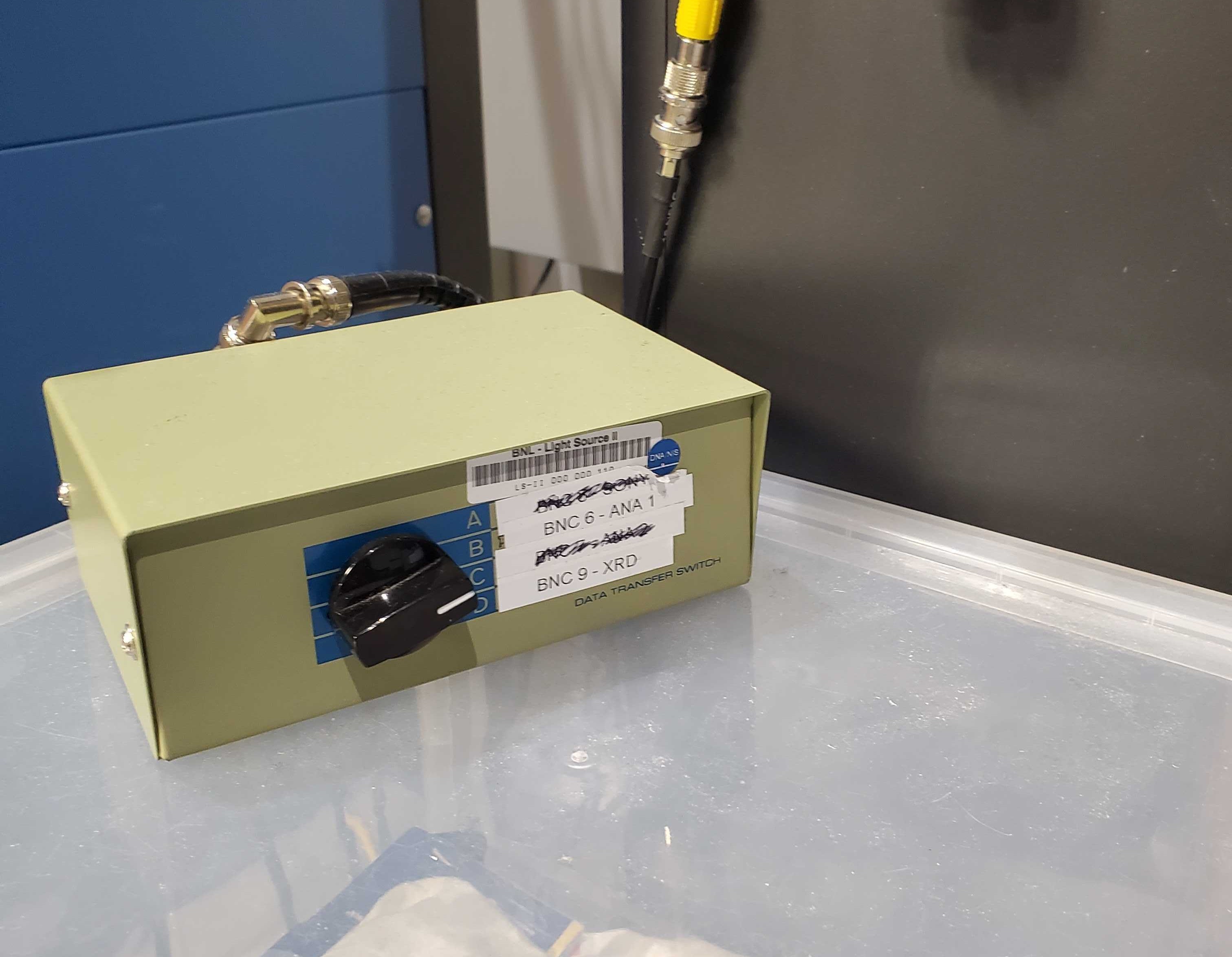
Fig. 4.3 (Left) The aligment pin mounted on the goniometer head. (Right) The switch for analog video signals.

Verify that the direct beam hits the camera, then evaluate the size and shape of the beam. You may want to apply some attenuation to the beam – the YAG crystal bleeds at high flux, making it hard to assess the actual size and shape of the beam.

RE(mv(attenuator, 2))

The beam should be a small oval with the axes of the oval parallel and perpendicular to gravity. If the oval is slanted, try adjusting the yaw of the focusing mirror (See Section 2.5.3), for example

RE(mvr(m2.yaw, 0.01))

With the shadow of the pin in the focused, direct beam, note its position on screen. Rotate the phi axis by 180 degrees. Note the new position. Find the center point of these two positions and move table.lateral to place the center of the beam at that center point using command like this:

RE(mvr(table.lateral, 0.25))

Rotate the chi circle by -90 degrees so that the pin is in the horizontal plane. Repeat the procedure of noting the position, rotating phi by 180 degrees, and finding the center point. Place the beam at the center point by doing

RE(mvr(table.vertical, 0.25))

Read and record the table motor positions.

See Section 2.4 for details of table movement.

Future Tech!

Direct beam camera that can be read via AreaDetector. Do image analysis on shadow of pin to compute correct table.vertical and table.lateral positions.

4.3. Slit alignment

Open the slits to their fully open position:

RE(mv(slits.hsize, 8))
RE(mv(slits.vsize, 8))

The direct beam should still be visible on the direct beam camera.

Note

What to do if the beam is not near the center of the slits?

To align and calibrate the goniometer slits, do

RE(align_slits())

The optional arguments to this plan are

nsteps

Number of steps in each scan (default is 31)

move

If True, move to the centroid (default is True)

calibrate

If True, reset offset so that centroid is at 0 (default is True)

inttime

Scan dwell time (default is 0.5 seconds)

The slit alignment procedure will run a linescan (Section 4.1) on each of the four slits individually, plotting the signal on the monitor versus slit position. This signal should be a step-like function, so the result is fit to an error function. The slit is moved to the centroid of the fitted error function and the offset of the slit is reset to define the zero position. The result of an individual slit scan looks like Figure 4.4.

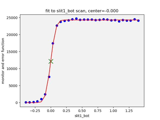
Fig. 4.4 The fit to an individual slit scan, in this case, bottom blade.

Once aligned and calibrated, the slit size for the experiment is set to 1 mm iun the horizontal and 0.12 mm in the vertical. This is the equivalent of

RE(mv(slits.hsize, 1))
RE(mv(slits.vsize, 0.120))

4.4. Horizontal detector alignment

With the beam in the center of the goniometer and in the center of the slits, we next align the Mythen with the direct beam. To do so, we perform a linescan of the dethor axis, moving the detector across the incident beam.

The attenuator needs to be set to a value suitable for the incident beam, something like:

RE(mv(attenuator, 6))

then perform a linescan of the dethor motor:

RE(linescan(dethor, 'mca_full', -3, 3, 61))

The live plot will show the progress of the scan. Once the scan is finished, some simple peak interpretation is performed, shown in Figure 4.5.

The peak-like shape is reduced to find the peak, the center of mass (the “com”), and the center of the full width at half maximum (the “cen”). In this case, dethor is moved to the cen value.

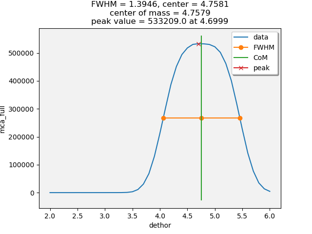
Fig. 4.5 Interpretation of the horizontal scan of dethor to center the Mythen on the incident beam.

At this point, take a count on the Mythen to find the position of the direct beam on the detector. Set the dwell_time to something short and do an exposure.

RE(mv(dwell_time, 0.1))
RE(count([mythen], 1))

The signal from the exposure will have a peak centered on some pixel. If the slits are 120 μm, then the direct beam will illuminate 3 or 4 strips, as the strip width is 50 μm, as shown on the Mythen2 specification sheet and there 1280 strips on the detector.

The direct beam should be around the 200^th strip. Adjust the gap on the flight path holder so that is approximately true. A simple calculation of the center of the illuminated area from the count will be good enough. This places the beam closer to the bottom of the detector, thus most of the strips are above the direct beam – also, then, the reflected beam in an XRR experiment. See Figure 4.6.

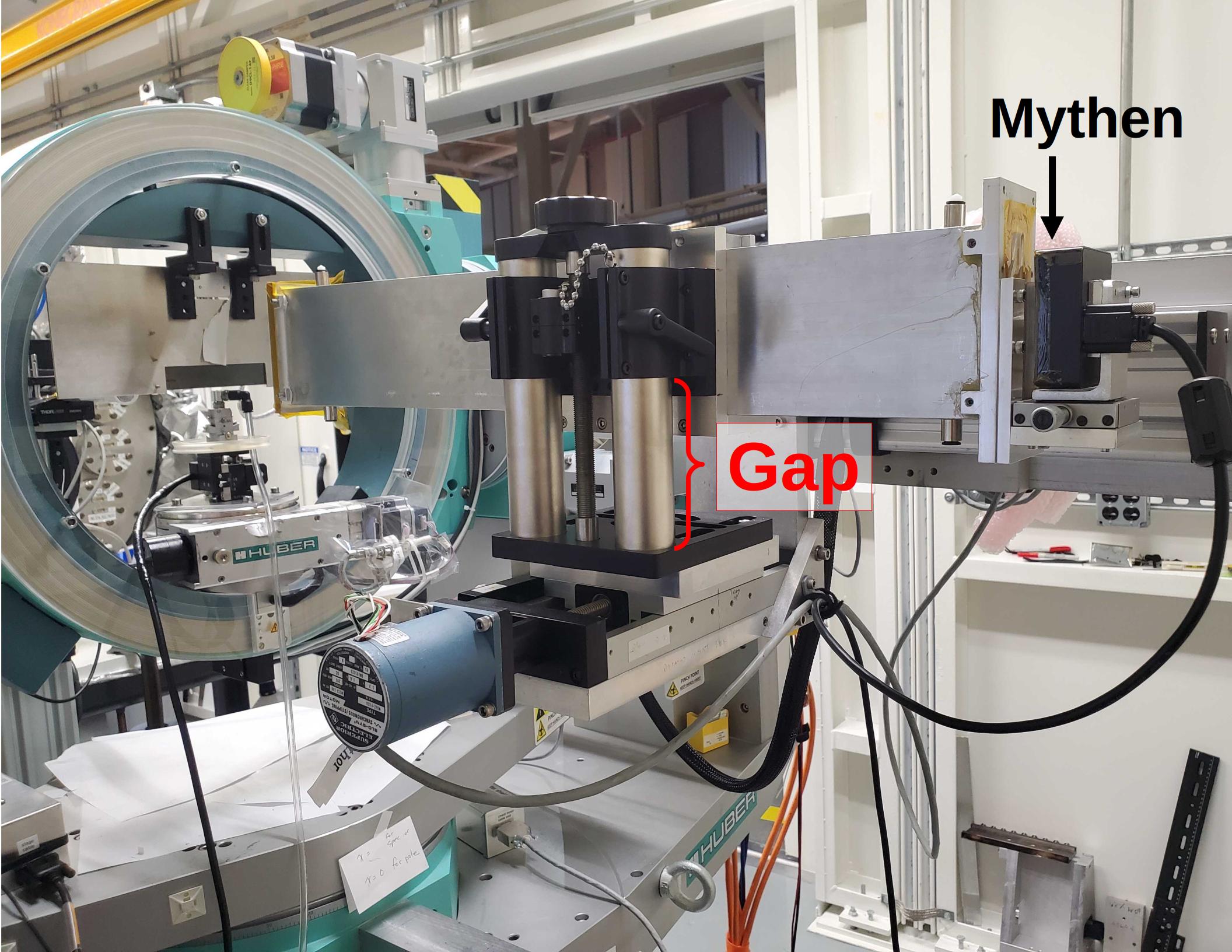
Fig. 4.6 The gap measures the elevation of the Mythen and its flight path on the hand-operated vertical jack.

4.5. Mythen Calibration

With the beam around strip 200, run a linescan of delta, plotting the signal from the full MCA spectrum from the Mythen. This will be dominated by the integral under the 3 or 4 strip wide peak due to the direct beam.

This scan will find the extent of the detector in delta. As the beam passes over the detector, the signal will be approximately constant.

Typical scan parameters are:

RE(mythen_calibration(-4, 1, 1001))

The optional arguments to mythen_calibration are:

start

From delta=0, the starting angle of the scan, in degrees

stop

From delta=0, the ending position of the scan, in degrees

nsteps

The number of steps in the scan

inttime

The dwell time at each point in the scan. Default is 0.1 seconds

force

When true, force the scan to run even if the beamline is not ready (e.g. no beam). Default is False.

The live plot will look something like Figure 4.7.

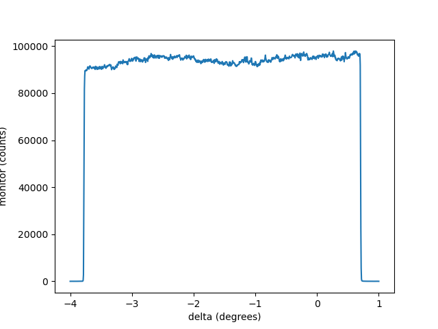
Fig. 4.7 A liveplot of the Mythen full MCA integration versus delta angle.

When the linescan in delta is finished, some data reduction happens and a report is generated. This report is written to the screen. It is also written to a PowerPoint file in the data folder. It’s contents look something like Figure 4.8.

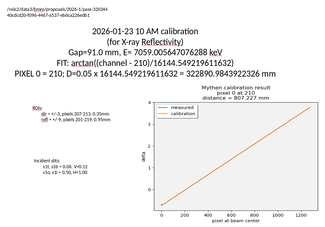
Fig. 4.8 An image of the PowerPoint report made on the Mythen calibration scan. (Note: there are some obvious errors in this picture. Picture will be updated once the report is fixed.)

In the upper right corner of this report, the path to the proposal folder is written as is the UID of the Tiled record. The numerical results of the fit are given in the main text. A plot of fit to the beam position on the detector is shown in the plot. Form this fit, we get the formula for mapping delta angle to direct beam detector position, as well as values for the gap, the distance form the goniometer eucentric to the detector, and the pixel underneath the direct beam at delta=0.

Once this analysis is finished, the ROIs for the direct and reflected beam are set. Those values and the slits sizes are also in the report.

You can visualize the ROIs over the direct beam spectrum by moving delta to 0, doing a count, then plotting the spectrum just counted.

RE(mv(delta, 0))
RE(count([mythen], 1))
mythen.plot(N)

The value of N in the mythen.plot function identifies which ROI will be shown in the plot.

mythen.plot(1)

This will show the full MCA spectrum ROI (ROI1), i.e. the entire detector

mythen.plot(2)

This will show the direct beam ROI (ROI2). As this is only a few strips wide, it is hard to see at full scale.

mythen.plot(3)

This will show the reflected beam ROI (ROI3). This is still quite narrow, but more apparent than the direct beam ROI.

You can specify the pixel range of this plot, e.g.:

mythen.plot(2, xmin=175, xmax=225)

Fig. 4.9 A zoomed-in view of the direct beam ROI on top of the MCA spectrum, made using mythen.plot(2).

As a final check of the instrument alignment and the setting of the detector ROIs, do a linescan with rather fine steps of delta.

RE(linescan(delta, 'mythen', -0.15, 0.15, 61))

The live plot will show the direct beam ROI and the wider, reflected beam ROI as functions of delta. The narrower direct beam ROI should be well centered within the reflected beam ROI. If it is not, then something about the instrument alignment or the setting of the ROIs was done incorrectly.

At the end of the scan, the direct beam peak is interpreted for peak, com, and cen positions. The offset of the delta motor is reset so that the cen is at 0. This should be a very small change in offset.

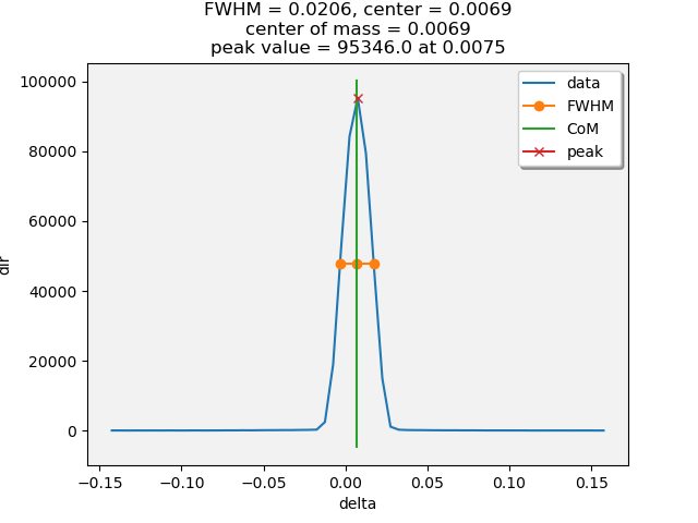
Fig. 4.10 (Left) Live plot of the scan of delta. (Right) Showing the interpretation of the direct beam ROI as a function of delta angle. This should be narrow and centered very close to 0. Note that the com and cen are at the same position. This is a good alignment!

4.6. Sample alignment

A sample for XRR is usually a large, flat wafer. The correct alignment has the sample surface parallel to the beam path and at a height such that it blocks half the beam. With that alignment, the center of the beam will be on the center of the sample as the incident angle changes and the beam will spread symmetrically over the length of the sample as the angle changes.

To find the correct vertical position – samplez – of the flat sample:

RE(sample_vertical())

The optional arguments to sample_vertical() are:

start

Starting point measured in mm from the current position of samplez. Default is -0.5.

stop

Ending point measured in mm from the current position of samplez. Default is 0.5.

nsteps

The number of steps in the scan. Default is 101.

inttime

The dwell time in seconds at each step of the scan. Default is 0.1 second.

Upon completion of the scan, an error function will be fit to the lineshape. The centroid of the lineshape will be the position of half intensity, i.e. where the sample is blocking half of the beam. samplez will be moved to that position.

Todo

Show a picture

To find the correct angular position – eta – of the flat sample:

RE(sample_eta())

start

Starting point measured in degrees from the current position of eta. Default is -0.25.

stop

Ending point measured in degrees from the current position of eta. Default is 0.25.

nsteps

The number of steps in the scan. Default is 51.

inttime

The dwell time in seconds at each step of the scan. Default is 0.1 second.

choice

A choice of how to select the zero of eta. The choices are:

• "peak": max signal value

• "com": the point of the center of mass of the signal

• "cen": center point of the full width at half max

• "crossing": crossing point of lines regressed to the two sides of the peak

Upon completion of the scan, all the peak statistics (peak, com, cen, and crossing) will be computed and reported on screen. The value of choice will be used to move eta to position. That position will be redefined in EPICS as the zero of ete.

Todo

Show a picture

Iteration of RE(samples_vertical()) and RE(sample_eta()) may be required.